visutils
# install packages if necessary
# devtools::install_github("cellgeni/visutils")
library(visutils)
# package to load h5ad file as Seurat objects
library(schard)
library(Seurat)
library(Matrix)
Download the data
We will use data from https://www.ebi.ac.uk/biostudies/arrayexpress/studies/E-MTAB-13084, lets first load metadata:
meta = read.table('https://ftp.ebi.ac.uk/biostudies/fire/E-MTAB-/084/E-MTAB-13084/Files/E-MTAB-13084.sdrf.txt',header = TRUE,check.names = FALSE,sep='\t',quote = '')
# samples are duplicated for each fastq, lets collapse them
colnames(meta) = gsub('Characteristics\\[|]','',colnames(meta))
meta = unique(meta[,c('Source Name','age','sex','sampling site','disease','sample id')])
meta$`body part` = splitSub(meta$`sample id`,'_',1)
rownames(meta) = meta$`Source Name`
ord = c(body=1,face=2,bcc=3)
meta = meta[order(ord[meta$`body part`]),]
meta[1:3,]
#>                             Source Name age  sex            sampling site disease       sample id body part
#> WSSKNKCLsp104466211 WSSKNKCLsp104466211  60 male                     back  normal     body_back1a      body
#> WSSKNKCLsp10446623   WSSKNKCLsp10446623  55 male inguinal part of abdomen  normal body_inguinal1a      body
#> WSSKNKCLsp10767965   WSSKNKCLsp10767965  47 male                  abdomen  normal  body_abdomen1b      body
We’ll take h5ad data from https://spatial-skin-atlas.cellgeni.sanger.ac.uk/ and load them using hchard package. These h5ad contains cell2location results so we will be able to use them. Alternatively visium data can be loaded from spaceranger output using Seurat::Load10X_Spatial or its wrapper visutils::myLoad10X_Spatial. In this case one will need to load cell2location predictions separately.
# download data to to temporary location and load as Seurat object
tmpfile = tempfile()
vs = list()
for(i in 1:nrow(meta)){
  tryCatch({
    download.file(paste0('https://cellgeni.cog.sanger.ac.uk/spatial-skin-atlas/download/',meta$`Source Name`[i],'.h5ad'),
                        tmpfile,quiet = TRUE)
    vs[[meta$`Source Name`[i]]] = schard::h5ad2seurat_spatial(tmpfile,use.raw = TRUE,img.res = 'hires')
    file.remove(tmpfile)
    cat('.')
  },warning=function(w){cat('!')})
}
#> !.............................
print('\n# spots:')
#> [1] "\n# spots:"
sapply(vs,ncol)
#> WSSKNKCLsp10446623 WSSKNKCLsp10767965 WSSKNKCLsp10767966 WSSKNKCLsp10767967 WSSKNKCLsp10767968 WSSKNKCLsp12887263 WSSKNKCLsp12887264
#>               1310               1755               1826               1632               1958               2097               2546
#> WSSKNKCLsp12887265 WSSKNKCLsp10446613 WSSKNKCLsp10446614 WSSKNKCLsp10446615 WSSKNKCLsp10446616 WSSKNKCLsp10446617 WSSKNKCLsp10446618
#>               2247                986                927               1547               1494               1552               1577
#> WSSKNKCLsp10446619 WSSKNKCLsp10446620 WSSKNKCLsp12140366 WSSKNKCLsp12140367 WSSKNKCLsp12140368 WSSKNKCLsp12140369 WSSKNKCLsp12887266
#>               1163               2036               1987                963               1642               1383               1344
#> WSSKNKCLsp12140270 WSSKNKCLsp12140271 WSSKNKCLsp12140272 WSSKNKCLsp12140273 WSSKNKCLsp12887267 WSSKNKCLsp12887268 WSSKNKCLsp12887269
#>                813               1043               1870               1200               1334               1148                932
#> WSSKNKCLsp12887270
#>                952
One sample is not on the portal, probably due to low quality, lets remove it from meta:
meta = meta[names(vs),]
table(meta$`body part`)
#>
#>  bcc body face
#>    8    8   13
Load spot annotation
In this tutorial we will look on celltype abundance in dependence on distance from dermis-to-epidermis junction which we will defined as epidermis spots that contact with dermis. Any set of spots can be used to define distance from. It can be defined semi-automatically as tissue border (see tissue border vignette elsewhere). We will use manual spot annotation made in loupe to define dermis-to-epidermis junction. Lets load it.
path2annot = '/nfs/cellgeni/pasham/projects/2303.bcc.skin/data.nfs/manuall.annotation/fixed/'
nspots = sapply(vs,ncol) # before filtering
for(i in 1:nrow(meta)){
  a = read.csv(paste0(path2annot,'/',meta$`Source Name`[[i]],'.csv'),row.names = 1)
  # subste to common spots (one that are not in annotation are empty)
  cmn = intersect(rownames(a),colnames(vs[[i]]))
  vs[[i]] = vs[[i]][,cmn]
  vs[[i]] = AddMetaData(vs[[i]],a[cmn,1],col.name = 'man.ann')
}
#> Warning: Not validating Seurat objects
#> Not validating Seurat objects
#> Not validating Seurat objects
#> Not validating Seurat objects
#> Not validating Seurat objects
#> Not validating Seurat objects
#> Not validating Seurat objects
#> Not validating Seurat objects
#> Not validating Seurat objects
#> Not validating Seurat objects
#> Not validating Seurat objects
#> Not validating Seurat objects
#> Not validating Seurat objects
#> Not validating Seurat objects
#> Not validating Seurat objects
#> Not validating Seurat objects
#> Not validating Seurat objects
#> Not validating Seurat objects
#> Not validating Seurat objects
#> Not validating Seurat objects
#> Not validating Seurat objects
#> Not validating Seurat objects
#> Not validating Seurat objects
#> Not validating Seurat objects
#> Not validating Seurat objects
#> Not validating Seurat objects
nspots - sapply(vs,ncol) # just few spots were removed
#> WSSKNKCLsp10446623 WSSKNKCLsp10767965 WSSKNKCLsp10767966 WSSKNKCLsp10767967 WSSKNKCLsp10767968 WSSKNKCLsp12887263 WSSKNKCLsp12887264
#>                  4                288                 33                 33                  2                 10                  0
#> WSSKNKCLsp12887265 WSSKNKCLsp10446613 WSSKNKCLsp10446614 WSSKNKCLsp10446615 WSSKNKCLsp10446616 WSSKNKCLsp10446617 WSSKNKCLsp10446618
#>                  4                  6                 39                  2                 15                  0                 16
#> WSSKNKCLsp10446619 WSSKNKCLsp10446620 WSSKNKCLsp12140366 WSSKNKCLsp12140367 WSSKNKCLsp12140368 WSSKNKCLsp12140369 WSSKNKCLsp12887266
#>                 24                  1                  4                 20                 15                 10                  9
#> WSSKNKCLsp12140270 WSSKNKCLsp12140271 WSSKNKCLsp12140272 WSSKNKCLsp12140273 WSSKNKCLsp12887267 WSSKNKCLsp12887268 WSSKNKCLsp12887269
#>                  3                  7                 12                  3                 12                 18                  9
#> WSSKNKCLsp12887270
#>                  0
Check data
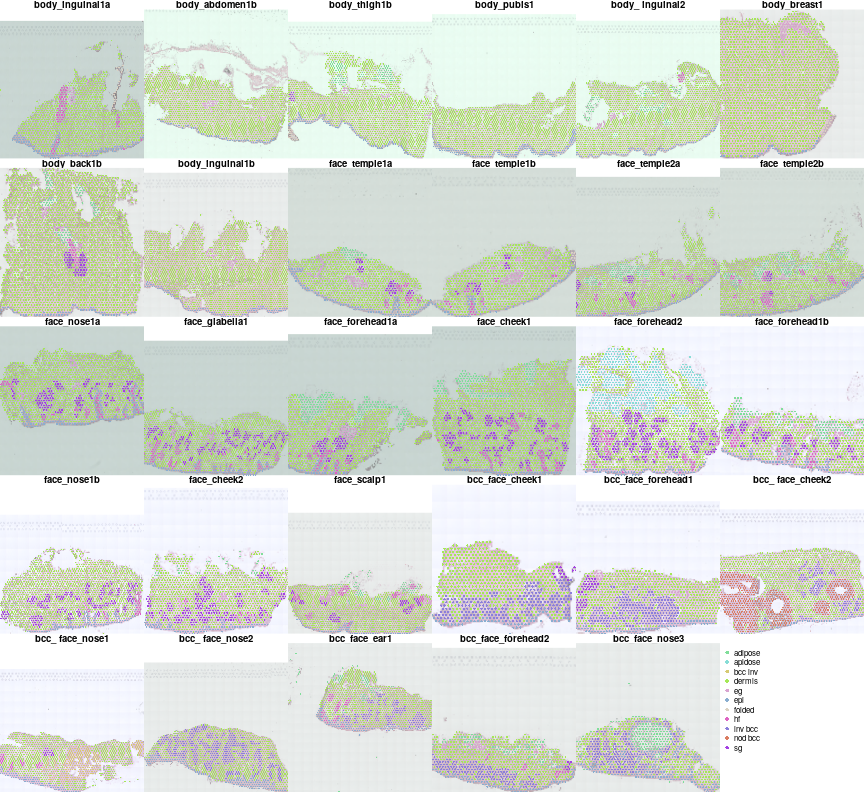
Lets check annotation first
ann2col = char2col(unlist(lapply(vs,function(v)v$man.ann)))
par(mfrow=c(5,6),mar=c(0,0,1,0),bty='n')
for(i in names(vs)){
  plotVisium(vs[[i]],vs[[i]]$man.ann,z2col=ann2col,main=meta[i,'sample id'],cex=0.6,he.img.width=200,plot.legend = FALSE,img.alpha=0.5)
}
plot.new()
legend('topleft',bty='n',col=ann2col,legend = names(ann2col),pch=16)
Define distance to e2d junction
We will analyse celltype abundance and gene expression in dependence on distance to dermis to epidermis junction.
for(i in names(vs)){
  t = defineJunction(vs[[i]],ann.column = 'man.ann',which='epi',contactTo = 'dermis')
  vs[[i]]@meta.data$junction = t$junction
  vs[[i]]@meta.data$dist2junction = t$dist2junction
}
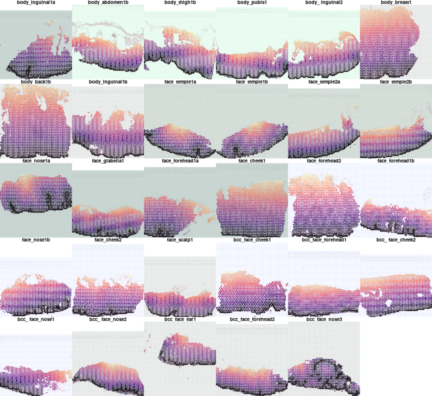
Lets plot distance to junction by color gradient and mark the junction by black border.
par(mfrow=c(5,6),mar=c(0,0,1,0),bty='n')
for(i in names(vs)){
  plotVisium(vs[[i]],abs(vs[[i]]$dist2junction),border=ifelse(vs[[i]]$junction,'black',NA),z2col = 'magma',
             main=meta[i,'sample id'],cex=0.7,he.img.width=200,img.alpha=0.5,plot.legend = FALSE)

}
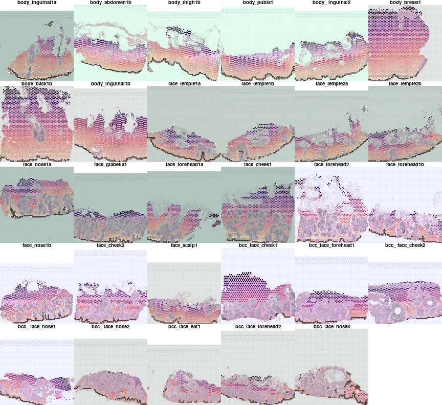
Samples contain some irregular structures such as hair follicle, lets focus for now on dermis and epidermis only and remove all spots that contact with anything else
par(mfrow=c(5,6),mar=c(0,0,1,0),bty='n')
ann2use = c('epi','dermis')
for(i in names(vs)){
  vs[[i]]$dist2unwanted = calcDistance2SpotSet(vs[[i]],!(vs[[i]]$man.ann %in% ann2use))
  plotVisium(vs[[i]],vs[[i]]$dist2junction,border=ifelse(vs[[i]]$junction,'black',NA),main=meta[i,'sample id'],cex=0.6,z2col='magma',
             he.img.width=200,img.alpha=0.7,plot.legend = FALSE,
             spot.filter = vs[[i]]$dist2unwanted > 1.2)

}
Differentiall analyses
Celltypes
Prepare summary matrix
There are still epidermis invaginations on temple sample that likely correspond to hair follicles. It is probably better to remove them but lets proceed as is for now. First lets prepare input data for the analyses and then use makeDistFeatureSampleTable to calculate mean normalized (per spot) celltype abundance. The function returns 3D matrix: distance * celltype * sample
# group cells to plot them in meaningfull order
celltypes = c('APOD+ fibroblasts'='4','BC'='4','Basal keratinocytes'='1','CD8+ T RM'='3','Chondrocytes'='4','DC1'='3','DC2'='3','IL8+ DC1'='3','ILC_NK'='3','LEC'='5',
'Macro1_2'='3','MastC'='3','Melanocytes'='2','MigDC'='3','Monocytes'='3','NK'='3','Neuronal_SchwannC'='4','POSTN+ fibroblasts'='4','PTGDS+ fibroblasts'='4',
'PlasmaC'='3','RGS5+ pericytes'='5','SFRP2+ fibroblasts'='4','SMC'='5','Skeletal muscle cells'='4','Suprabasal keratinocytes'='1','T reg'='3','TAGLN+ pericytes'='5',
'Tc'='3','Th'='3','VEC'='5')
celltypes = data.frame(celltype=names(celltypes),class=celltypes)
# extract spot information and combine into single data.frame
spots = do.call(rbind,lapply(vs,function(v)v@meta.data))
# subset cell2location results
c2lm = spots[,grep('c2l_',colnames(spots))]
colnames(c2lm) = sub('c2l_','',colnames(c2lm))

# binarise the distance
spots$dist2junction = round(spots$dist2junction)
# we will use only dermis and epidermis and dismiss all spots that contact other features, plus we will consider only two spot layers on epidermis and 12 in dermis
spot.filter = spots$dist2unwanted > 1.2 & spots$dist2junction > -12 & spots$dist2junction < 2
# lets calculate matrix with average celltype abundances for each distance bin and each sample
dfsmtx.c2l = makeDistFeatureSampleTable(dist = spots$dist2junction,
                                    sample = spots$library_id,
                                    data = c2lm,
                                    per.spot.norm = TRUE,
                                    f = spot.filter)
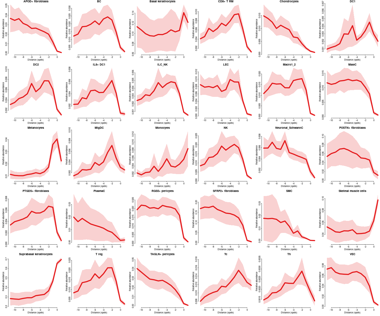
Celltype distribution across all dataset
par(mfrow=c(5,6),mar=c(3,3,1,0),bty='n',tcl=-0.2,mgp=c(1.3,0.3,0),oma=c(0,0,0,0))
for(ct in celltypes$celltype)
  plotFeatureProfiles(dfsmtx.c2l,features=ct,cols = "#E41A1C",lwd=5,main=ct,legend. = FALSE,scaleY=FALSE)
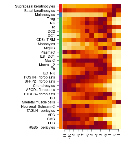
or one can summarise it as heatmap
# clalculate cross-sample mean celltype abundance
m = apply(dfsmtx.c2l,1:2,mean,na.rm=TRUE)
# max-norm per celltype
m = sweep(m,2,apply(m,2,max),'/')
celltypes = celltypes[order(celltypes$class,-apply(m,2,which.max),decreasing = T),]
par(mar=c(4,15,1,1),bty='n')
imageWithText(m[,celltypes$celltype],'',rowAnns = list(celltypes$class),rowAnnCols = list(char2col(celltypes$class)))
Compare body vs face
Lets compare body against face, testTDConditions performs t.test comparing two conditions for each celltype and each distance
comp.c2l = testTDConditions(dfsmtx.c2l,meta$`body part`=='body',meta$`body part`=='face')
Visualize results
# reorder celltypes by depth of max abundance in body
celltypes = celltypes[order(celltypes$class,-apply(comp.c2l$m1,2,which.max),decreasing = T),]
par(mfrow=c(1,3),mar=c(4,11,1,4))
# order cells by class and then by location
plotTD.HM(comp.c2l,fdr.thrs = c('x'=0.05,'*'=0.2,'.'=0.5),order = celltypes$celltype,cond.titles = c('body','face'),feature.class = celltypes$class)
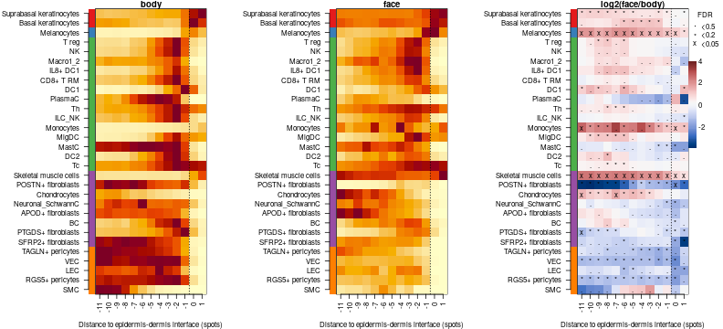
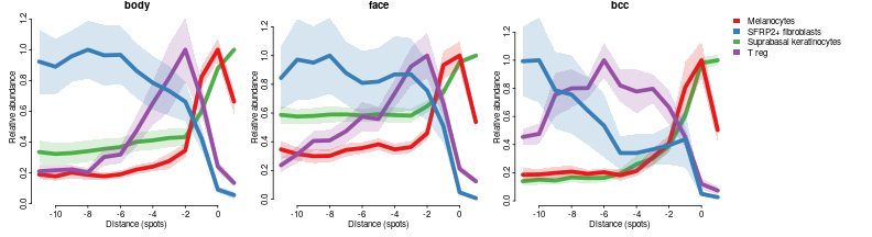
The plot above shows two types of information. First it gives spatial (along distance to dermis to epiderms junction) distribution of different cell types in two conditions, then it tells which celltypes and at which distance are significantly more abundant in face compared to body. For example it clearly shows that Suprabasal keratinocytes are most superficial celltype followed by Basal kertinocytes and Melanocytes then by immune cell types and fibroblats. Lets illustrate it by profile plots:
celltypes=c('Suprabasal keratinocytes','Melanocytes','T reg','SFRP2+ fibroblasts')
cols = char2col(celltypes)
par(mfrow=c(1,3),mar=c(3,3,1,0),bty='n',tcl=-0.2,mgp=c(1.3,0.3,0),oma=c(0,0,0,14))
for(bp in c('body','face','bcc'))
  plotFeatureProfiles(dfsmtx.c2l[,,meta$`body part`==bp],features=celltypes,cols = cols,lwd=5,sd.mult = 1,legend. = bp=='bcc',main=bp)
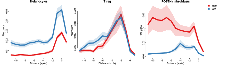
In terms of differential abundance it shows that melanocytes, and T reg are enriched, while POSTN+ fibroblasts are depleted in face compared to body:
celltypes=c('Melanocytes','T reg','POSTN+ fibroblasts')
cols = char2col(c('face','body'))
par(mfrow=c(1,3),mar=c(3,3,1,0),bty='n',tcl=-0.2,mgp=c(1.3,0.3,0),oma=c(0,0,0,14))
for(ct in celltypes)
  plotConditionsProfiles(dfsmtx.c2l,feature=ct,meta$`body part`,cols = cols,lwd=5,sd.mult = 1,legend. = ct==celltypes[length(celltypes)],main=ct)
Gene expression
Select genes to work with
Lets now look on gene expression, first log-normalize expression and select highly variable genes in per-sample manner
vs = lapply(vs,NormalizeData,verbose=FALSE)
vs = lapply(vs,FindVariableFeatures,verbose=FALSE)
For time sake we will use only genes that are highly variable in at least 20 samples, this threshould can be relaxed in real-live applications:
hvg = table(unlist(lapply(vs,VariableFeatures)))
barplot(table(hvg))
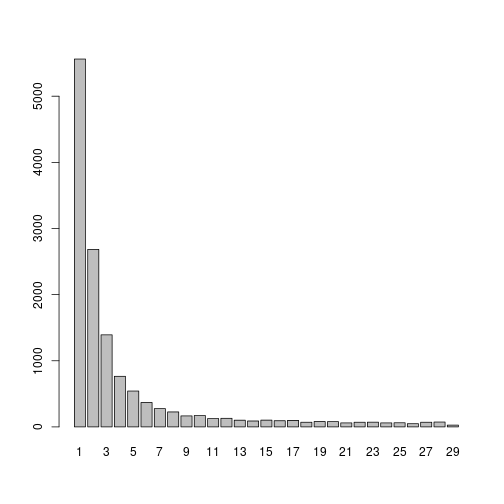
hvg = names(hvg)[hvg>=10]
length(hvg)
#> [1] 1682
Lets assemble expression matrix for all spots and selected genes
lcpm = do.call(cbind,lapply(vs,function(v)v[['Spatial']]$data[hvg,]))
lcpm = Matrix::t(lcpm) # since it is sparse matrix we need t from Matrix package
Prepare summary matrix
Now we can summarise gene expression in the same way we did with cell type abundance. It is advantageous to use multiple cores since with many genes it can take quite a while.
doMC::registerDoMC(2)
dfsmtx.ge = makeDistFeatureSampleTable(dist = spots$dist2junction,
                                    sample = spots$library_id,
                                    data = lcpm,
                                    per.spot.norm = FALSE,
                                    f = spot.filter,
                                    ncores=4)
Compare body vs face
Now lets test differential expression between face and body
comp.ge = testTDConditions(dfsmtx.ge,meta$`body part`=='body',meta$`body part`=='face')
Lets check how genes are distributed by number of distance bin with significant changes (fdr < 0.05 & fold change > 2)
comp.ge$sgn = comp.ge$fdr<0.05 & abs(comp.ge$m2-comp.ge$m1) >= log(2)
table(apply(comp.ge$sgn,2,sum))
#>
#>    0    1    2    3    4    5    6    7    8    9   10   11   12   13
#> 1563   24   12   12    8    1    2    7   10   10   10    7    5   11
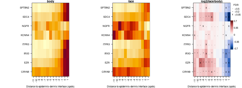
Visualize results
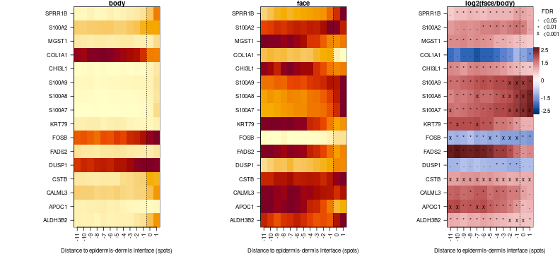
Now we can plot gene expression as heatmaps. We will make fdr cutoff stronger to highlight more significant genes. There is not need to take log, since analyses was done already on log CPM, so we will set log to FALSE.
par(mfrow=c(1,3),mar=c(4,11,1,4))
f = order(apply(comp.ge$sgn,2,sum),decreasing = TRUE)[1:16]
comp.ge.f = lapply(comp.ge,function(x)x[,f])
plotTD.HM(comp.ge.f,fdr.thrs = c('x'=0.001,'*'=0.01,'.'=0.05),cond.titles = c('body','face'),log=FALSE)
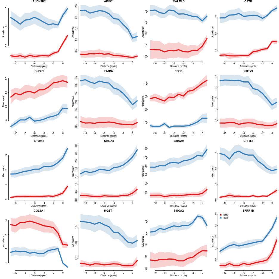
We can also plot profiles for individual genes
genes=colnames(comp.ge.f$pv)
cols = char2col(c('body','face'))
par(mfrow=c(4,4),mar=c(3,3,1,0),bty='n',tcl=-0.2,mgp=c(1.3,0.3,0),oma=c(0,0,0,0))
for(gn in genes[1:min(16,length(genes))]){
  leg = FALSE
  if(gn==genes[min(16,length(genes))])
    leg = list(x='topleft')
  plotConditionsProfiles(dfsmtx.ge,feature=gn,meta$`body part`, cols = cols,lwd=5,sd.mult = 1,
                         legend. = leg,main=gn)
}
Or plot spatial expression, APOC1 exhibits clearly higher expression in face compared to body
gene='APOC1'
par(mfrow=c(5,5),mar=c(0,0,1,4),bty='n',tcl=-0.2,mgp=c(1.3,0.3,0),oma=c(0,0,0,0))
o = order(meta$`body part`)
zlim = range(unlist(lapply(vs,function(v)v[['Spatial']]$data[gene,])))
for(s in meta$`Source Name`[o][meta$`body part`[o] != 'bcc'])
  plotVisium(vs[[s]],vs[[s]][['Spatial']]$data[gene,],z2col='magma',main=meta[s,'sample id'],legend.args = list(title=gene),he.img.width=200,
             spot.filter = vs[[s]]$man.ann %in% c('epi','dermis'),zlim=zlim,type='hex')
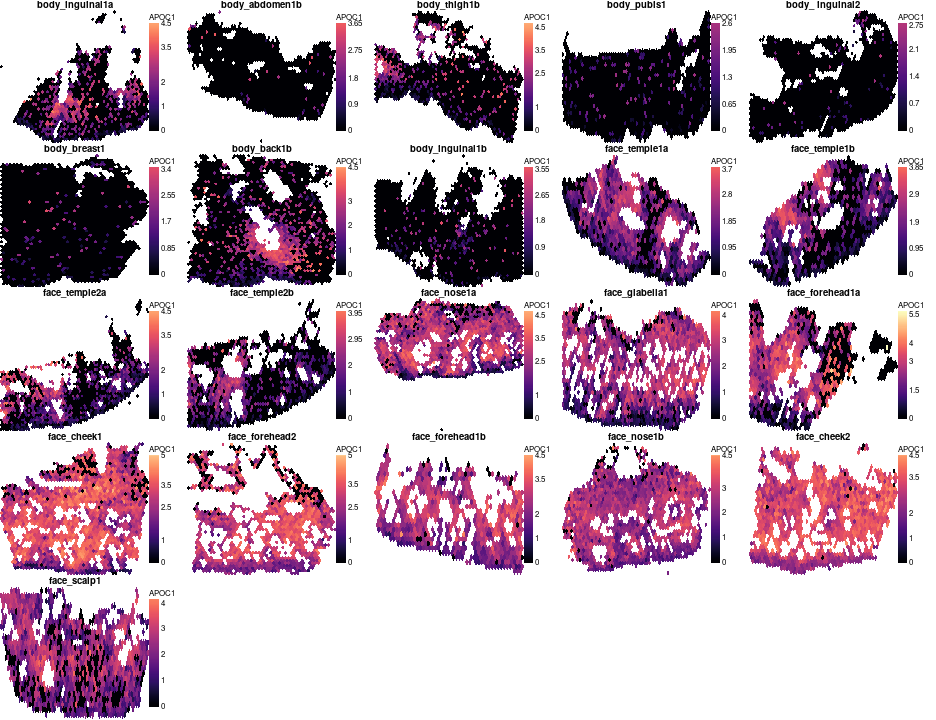
APOC1 does’n show clear spatial differences in expression, so lets look for genes that are higher in face at some distance to junction but lower at another:
sgnp = comp.ge$fdr<0.05 & (comp.ge$m2-comp.ge$m1) >=  0
sgnm = comp.ge$fdr<0.05 & (comp.ge$m2-comp.ge$m1) <=  0
par(mfrow=c(1,3),mar=c(4,11,1,4))
f = apply(sgnp,2,sum,na.rm=T) > 0 & apply(sgnm,2,sum,na.rm=T) > 0
comp.ge.f = lapply(comp.ge,function(x)x[,f])
plotTD.HM(comp.ge.f,fdr.thrs = c('x'=0.05,'*'=0.2,'.'=0.5),cond.titles = c('body','face'),log=FALSE)
Plot same genes as profiles
genes=colnames(comp.ge.f$pv)
cols = char2col(c('body','face'))
par(mfrow=c(2,3),mar=c(3,3,1,0),bty='n',tcl=-0.2,mgp=c(1.3,0.3,0),oma=c(0,0,0,0))
for(gn in genes[1:min(6,length(genes))])
  plotConditionsProfiles(dfsmtx.ge,feature=gn,meta$`body part`, cols = cols,lwd=5,sd.mult = 1,main=gn,legend.=list(x='topleft'))
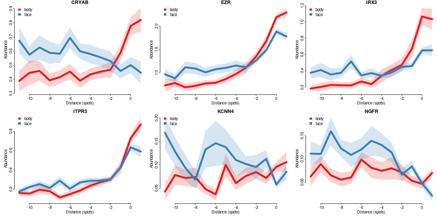
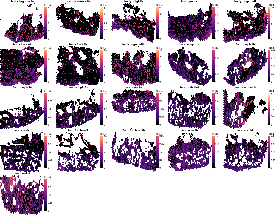
SDC4 expression is not very high, but it clearly show a tendency to be more superficial in body and be more evenly expressed in face.
gene='SDC4'
par(mfrow=c(5,5),mar=c(0,0,1,4),bty='n',tcl=-0.2,mgp=c(1.3,0.3,0),oma=c(0,0,0,0))
o = order(meta$`body part`)
zlim = range(unlist(lapply(vs,function(v)v[['Spatial']]$data[gene,])))
for(s in meta$`Source Name`[o][meta$`body part`[o] != 'bcc'])
  plotVisium(vs[[s]],vs[[s]][['Spatial']]$data[gene,],z2col='magma',main=meta[s,'sample id'],legend.args = list(title=gene),he.img.width=200,
             spot.filter = vs[[s]]$man.ann %in% c('epi','dermis'),zlim=zlim,type='hex')